M2 Lecture Notes: A Historical Journey through Mechanics

M2 Lecture Notes: A Historical Journey through Mechanics

Author: WANG Yizi

A Brief History of Kinematics: The Science of Motion

Historical Context

Kinematics, the study of motion without considering its causes, has roots in ancient astronomy. Early astronomers like Ptolemy described the motions of planets using complex geometric models. However, quantitatively studying velocity and acceleration was not a simple task. Before the invention of calculus, mathematicians struggled to describe instantaneous velocity.

A significant breakthrough came from the Merton School of philosophers at Oxford University in the 14th century. They were among the first to try to quantify accelerated motion. They developed the Mean Speed Theorem, which states that a body moving with constant acceleration travels the same distance as a body moving at a constant velocity equal to its mean velocity. This was a crucial step towards the “suvat” equations we use today.

The modern understanding of kinematics was forged during the Renaissance. Galileo Galilei (1564–1642), through his experiments with falling objects and projectiles, was one of the first to use mathematics to describe the trajectory of objects. His work laid the foundation for Newton’s laws of motion.

Review of M1 Kinematics

In M1, you focused on the motion of particles in a straight line with constant acceleration. You used the “suvat” equations:

• $v = u + at$
• $s = ut + \frac{1}{2}at^2$
• $v^2 = u^2 + 2as$
• $s = \frac{1}{2}(u+v)t$

You also analyzed motion using displacement-time and velocity-time graphs.

What to Expect in M2 Kinematics

In M2, we expand from one-dimensional to two-dimensional motion, and we move beyond constant acceleration.

• Projectile Motion: We will analyze the motion of particles under gravity in a vertical plane. This is a direct application of the M1 suvat equations, but now applied independently to the horizontal and vertical components of motion.
• Variable Acceleration: We will use calculus to describe motion where acceleration is not constant. You will learn to differentiate displacement with respect to time to find velocity, and differentiate velocity to find acceleration. Conversely, you will integrate acceleration to find velocity and integrate velocity to find displacement.
• Vectors: We will use vectors to represent displacement, velocity, and acceleration in a plane, for instance $\mathbf{r}(t) = t^2\mathbf{i} + \frac{1}{2}t^3\mathbf{j}$.

A Brief History of Statics: The Science of Equilibrium

Historical Context

Statics is the oldest branch of mechanics, with its principles first formally studied by Archimedes (c. 287–c. 212 BC). He rigorously developed the law of the lever and used it to calculate the centers of gravity of various shapes. His famous quote, “Give me a place to stand, and I shall move the Earth,” illustrates the power of levers and moments. His work was so foundational that it remained the standard for over 1800 years. Later, figures like Leonardo da Vinci (1452–1519) also studied forces, particularly in the context of building and engineering, but it was Archimedes who laid the mathematical groundwork for the entire field of statics.

Review of M1 Statics

In M1, you studied the equilibrium of a single particle. The key principle was that for a particle to be in equilibrium, the vector sum of all forces acting on it must be zero ($\Sigma \mathbf{F} = \mathbf{0}$). You applied this by resolving forces into perpendicular components—often horizontally and vertically, or parallel and perpendicular to a slope—and setting the sum of each component to zero. You became familiar with various types of forces: weight, normal reaction, tension in strings, and friction. You also learned the model for friction, where for a body in limiting equilibrium, the frictional force is related to the normal reaction by the coefficient of friction ($F \leq \mu R$). While moments are a central topic in M2, you were briefly introduced to them in M1 in simple cases of equilibrium for a body under the action of coplanar parallel forces.

What to Expect in M2 Statics

In M2, we move from particles to rigid bodies—objects with size and shape that do not deform.

• Moments: The concept of a moment (or torque) becomes crucial. For a rigid body to be in equilibrium, not only must the net force be zero, but the net moment about any point must also be zero ($\Sigma M = 0$). This prevents rotation.
• Centres of Mass: You will learn to find the center of mass for various uniform shapes (laminae) and composite bodies. The center of mass is the point where the entire weight of the body can be considered to act.
• Equilibrium of Rigid Bodies: You will solve problems involving ladders leaning against walls, objects suspended from points, and other scenarios where both force and moment equilibrium must be considered.

A Brief History of Dynamics: The Science of Caused Motion

Historical Context

Dynamics, the study of how forces cause motion, was revolutionized by Sir Isaac Newton (1643–1727). Before Newton, the understanding of motion was largely descriptive. Newton, with his three laws of motion published in his Principia Mathematica in 1687, created a predictive and mathematical framework. This was a monumental achievement that unified celestial and terrestrial mechanics—the same laws described both the orbit of the Moon and the trajectory of a cannonball. The concepts of work and energy, which you will study in M2, were developed later. Scholars like Gottfried Leibniz, and later Joseph-Louis Lagrange and William Rowan Hamilton, developed these ideas into powerful alternative formulations of mechanics.

Review of M1 Dynamics

In M1, you were introduced to Newton’s Second Law ($\mathbf{F} = m\mathbf{a}$) for a particle. You applied this fundamental law to a variety of problems, including particles on inclined planes (both smooth and rough) and systems of connected particles, where you analyzed two masses joined by a string, often involving a smooth pulley. You also studied momentum and impulse in one dimension, using the impulse-momentum principle ($I = mv - mu$) and the principle of conservation of momentum for two particles colliding directly.

What to Expect in M2 Dynamics

M2 significantly deepens the study of dynamics.

• Work and Energy: You will be introduced to the concepts of kinetic energy ($\frac{1}{2}mv^2$) and potential energy ($mgh$). The work-energy principle provides a powerful alternative method for solving dynamics problems.
• Collisions: We will revisit collisions, but now with more detail. You will learn about Newton’s Law of Restitution and the coefficient of restitution ($e$), which quantifies the “bounciness” of a collision. You will also calculate the loss of mechanical energy in impacts.
• Momentum as a Vector: Momentum and impulse will be treated as vectors, allowing you to solve more complex, two-dimensional problems.

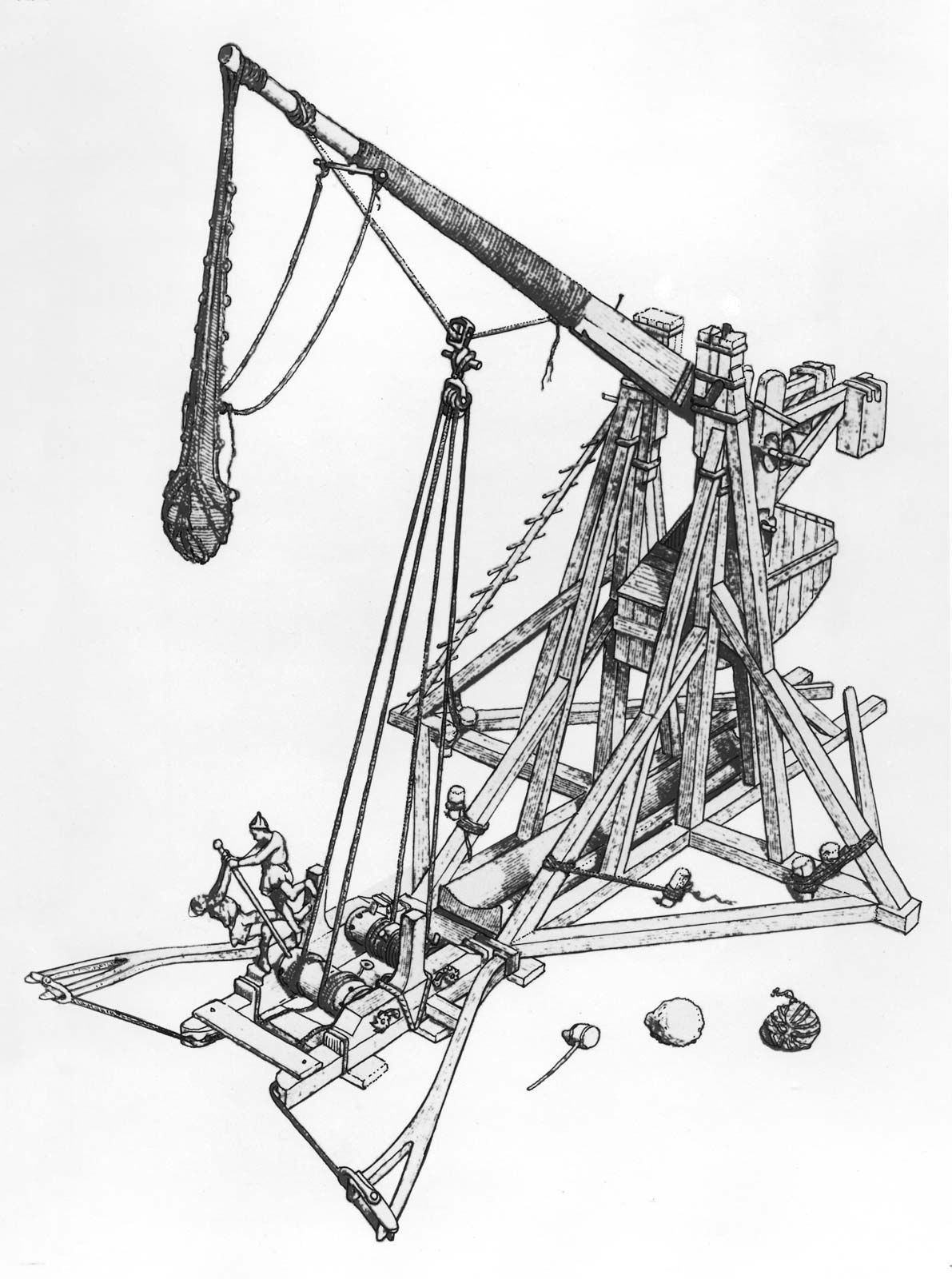
M2 Introduction Case Study: Analyzing a Medieval Trebuchet

To see how the different branches of mechanics come together, let’s consider a fascinating piece of medieval engineering: the trebuchet. A trebuchet uses a large counterweight to launch a projectile from a sling. Analyzing its design and operation provides a perfect preview of how we will integrate Kinematics, Statics, and Dynamics in M2.

Statics: Building the Machine

Before the trebuchet fires, it is a static structure. The primary concern for its designers was ensuring it was stable and strong enough to handle the immense forces involved.

• Equilibrium of Rigid Bodies: The entire frame of the trebuchet must be in equilibrium. We need to analyze the forces acting on it—the weight of the components, the tension in the ropes, and the reactions from the ground. In M2, you’ll learn to use the principles of moments ($\Sigma M=0$) and forces ($\Sigma F=0$) to ensure the structure doesn’t tip over or collapse. For example, we could determine the necessary width of the base to prevent it from tipping when the massive counterweight is lifted into its firing position.
• Centres of Mass: To analyze the stability, we need to know where the center of mass of the entire structure is, as well as the center of mass of individual components like the throwing arm. In M2, you will learn techniques to calculate the center of mass for composite bodies, which is essential for this kind of analysis.

Dynamics: The Firing Process

The moment the trebuchet is fired, it becomes a dynamic system. The goal is to transfer energy from the falling counterweight to the projectile as efficiently as possible.

• Work and Energy: This is a classic work-energy problem. The gravitational potential energy of the raised counterweight is converted into the kinetic energy of the throwing arm and, ultimately, the projectile. In M2, you will use the work-energy principle to analyze this energy transfer. We could ask questions like: How does the mass of the counterweight affect the launch speed of the projectile? How is energy lost to friction or air resistance?
• Collisions and Momentum: While not a direct collision in the M2 sense, the principles of momentum transfer are key. The rapid change in motion involves large forces and impulses. Understanding how momentum is transferred through the system is a core part of dynamics.

Kinematics: The Projectile’s Flight

Once the projectile leaves the sling, it is no longer connected to the machine. Its flight through the air is purely a kinematics problem.

• Projectile Motion: The path of the projectile is a classic example of projectile motion, which you will study in detail in M2. We can model its trajectory using the equations of motion under gravity.
• Vectors and Calculus: We can describe the projectile’s position, velocity, and acceleration at any moment using vectors. By applying calculus, we can answer key questions for the trebuchet’s operators: What is the optimal release angle to achieve the maximum range? How long will the projectile be in the air? What will its impact velocity be?

Summary

The trebuchet shows us that a single engineering problem requires all three pillars of mechanics. Statics ensures the machine is stable, dynamics describes the powerful energy transfer during firing, and kinematics predicts the outcome of the launch. This is a great example of the integrated problem-solving you will develop in M2.